Hydraulic fracturing teams may soon be able to achieve almost perfect proppant distribution across clusters in a stage, an advance that will significantly improve wells’ initial and long-term production. The key is autonomous intelligent fracturing, a novel technique that combines automated fleet operations with real-time measurements and lightning-fast modeling to fine-tune completion parameters during each stage.

Hess’ vision for AIF is ambitious. Realizing this vision will require substantial investments and close collaboration between multiple parties to develop new capabilities. For example, we will need more economic tools for evaluating fracture networks’ length and morphology and estimating how much fluid and proppant enters each cluster. To make useful recommendations based on this information, we will need to create faster models that still provide accurate predictions. And to implement those models’ recommendations, we must have reliable ways to control fracture geometry that can be deployed automatically.

In AOGR’s August issue, we detailed Hess’ approach to autonomous intelligent fracturing and explored steps it is taking to make AIF a reality. This article will explain why real-time frac optimization justifies that effort by looking at one of its biggest benefits: the potential production increase from near-perfect proppant distribution.

Huge Uplift

The gains can be substantial. When AIF’s real-time optimization is applied to a well that already would have strong proppant distribution using today’s techniques, it increases first-year production by at least 6%. For more problematic wells that otherwise would have uneven proppant distribution, the increase in first-year production tends to be around 20%.

To reach these estimates, Hess and ResFrac conducted two modeling studies comparing today’s stages to near-perfect ones. The first study involved a fully coupled hydraulic fracture reservoir simulation model, while the second looked at a much simpler fracture-reservoir simulation model to ensure the learnings were not model-dependent.

The fully coupled model was calibrated using a comprehensive dataset from Hess’ Observation Lateral project in the Bakken. Conducted in 2019 and 2020, the project studied how various completion designs influence fracture geometry and drainage. It took place on a six-well pad containing a 10,000-foot observation lateral through the Three Forks formation that was equipped with cemented pressure gauges and fiber optics. An offset lateral in the middle Bakken used fiber optics to gather cluster-level completion measurements and detect frac hits. A second offset housed geophones to enable microseismic mapping.

In any case, the fully coupled model accurately reproduced the fracture geometry, morphology and unique fracture pressure behavior from the observation lateral’s gauges. The reservoir model was calibrated to match the production history, bottom-hole pressure behavior and drainage pressures. The calibration process resembles the one illustrated in SPE 209164, “Observation Lateral Project: Direct Measurement of Far-Field Drainage in the Bakken,” though that paper discusses a loosely coupled model rather than a fully coupled one.

To check whether the conclusions drawn from the fully coupled model depend on the details of the Observation Lateral site’s fracture geometry, Hess and ResFrac conducted a second study that paired the same reservoir simulation model with a much simpler fracture model. The simple model specified fracture geometries based on rules of thumb rather than trying to deduce geometries from detailed data.

Specifically, the simple model calculated fracture lengths using cluster-level fluid volumes, then estimated the propped length to be a percentage of the total length. The model assumed that fracture conductivity rose in proportion to cluster-level fluid volumes, though it did account for fracture conductivity falling with effective normal stress.

The results from the simpler model should be less accurate than the ones from the fully coupled model. However, it is realistic enough to compare with the more robust model’s predictions and ensure that the learnings are not model-dependent.

Scenarios Considered

All the models were scaled down “sectors” to reduce runtime. The models included five Middle Bakken wells and 1,200-foot lateral sectors with 33-foot cluster spacing (36 clusters total). The fully coupled model simulated three stages with 12 clusters in each stage. Treatment designs were held constant at 1,000 barrels of fluid and 40,000 pounds of proppant for each cluster using a 50/50 mixture of 100-mesh and 40/70 sand. To evaluate the impact of well spacing on the perfect frac stage’s value, we modeled four spacings: 440 feet, 660 feet, 880 feet and 1,100 feet.

For the uniformity index, a measure of how evenly fluid is distributed across the clusters in a stage, we looked at three scenarios. The base case had a UI around 0.75, the average reported by Hess’ distributed acoustic sensing. A standard deviation of 0.09 was applied to ensure variations in the model UI matched the DAS measurements.

To quantify the impact of very poor uniformity, we also modeled a low-case UI around 0.25. Because variations are likely to be more extreme as uniformity falls, we set the standard deviation for this scenario to 0.22. This case highlights the cost of poor performance resulting from problems, such as plug failures, crossflow outside the casing stemming from poor cement, insufficient limited entry, etc.

Finally, we get to the star of the show. To model a near-perfect frac stage, we assumed a UI of 0.95 or higher and a standard deviation of 0.04 or lower. This UI reflects the reality that even the best completion is unlikely to achieve truly even distribution.

To generate scenarios with different uniformity indices, we changed: (a) the random variance in initial perforation diameter, and (b) constants that affect the magnitude of perforation erosion. The near-perfect UI scenario assumed a uniform initial perforation diameter and zero erosion.

The modeling assumed that proppant placed in each cluster is proportional to the cluster-level fluid volume. Recent studies suggest that cluster-level proppant distribution may differ significantly from fluid distribution because of nuances in how proppant transport occurs within the wellbore. Those nuances have not yet been studied enough for their impact to be considered here.

Model Predictions

Figure 1 shows examples of the fracture geometries (upper graphics) and drainage patterns (lower graphics) predicted by the fully coupled model. The left side shows the uniform fracture lengths and drainages we would expect from a near-perfect UI. The base case is less uniform, and the low case has highly variable fracture lengths and uneven drainage patterns.

FIGURE 1

Fracture Geometries (top) and Drainage Patterns (bottom) from Fully Coupled Model

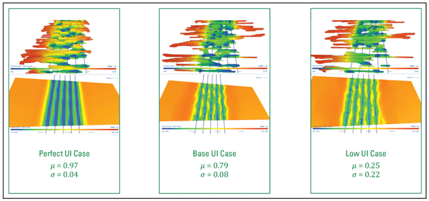
FIGURE 2

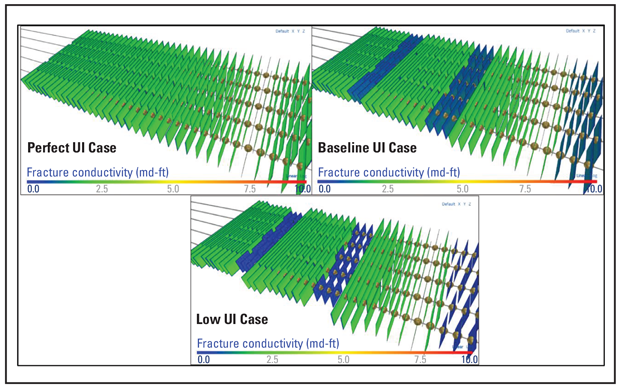
Example Fracture Lengths and Conductivities for the Simple Model

The negative effect of low UI on depletion is partially mitigated by well-to-well interaction. Regions with less fracture placement have weaker stress shadowing, making it somewhat more likely that fractures from adjacent wells will propagate into those regions.

Figure 2 shows an example of the input fracture lengths and conductivities used in the simple modeling study. With this simple approach, perfectly uniform fracture lengths and conductivities can be input into the reservoir model. A heel bias in fluid distribution was assumed for the base and low UI cases, resulting in shorter fractures in the toe cluster and longer fractures in the heel clusters. The simple model shows much less heterogeneity in fracture geometry compared with the fully coupled model, which was a goal of the comparison.

FIGURE 3

Impact of UI on First-Year Production

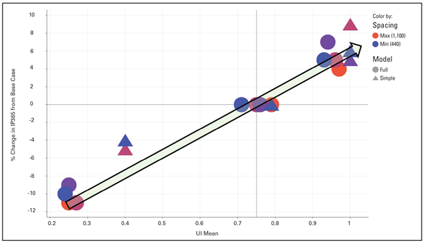
Of course, the point of these studies is to understand the perfect frac stage’s impact on production and economics. Figure 3 shows UI’s effect on one-year cumulative production in both models, with the fully coupled model represented by dots and the simple model represented by triangles. While the figure includes all four well spacings and differentiates them by color, some of the symbols are hidden by similar results in other spacing scenarios.

The production results are presented as a percentage of the base case UI production, with the base case results on the 0% line (y-axis). The UIs for each case in the fully coupled model vary somewhat because of the distribution of parameters used to simulate the different UIs in each model. The UIs for each UI group in the simple model are the same, since they are input parameters.

The results from the fully coupled model and simple model follow the same trend, suggesting the learnings from this work are not dependent on the model.

Although the results vary somewhat, the general trend is clear, showing a range in one-year production of about 20%. If UI can be increased from 0.25 to 0.75, the models indicate that first-year production will increase 10%. The gains from further improvements in UI fall as average UI improves, with first-year production increasing about 6% when UI jumps from the base case of 0.75 to almost 1.00.

The benefits of improving UI also diminish as production time increases. For example, the simulations show an increase of 10% in 10-year cumulative oil production when UI rises from 0.25 to 0.90-1.00.

The economic impact of variations in UI was estimated using typical Bakken well costs and evaluation parameters. Net present value is based on 10-year production. The economic inputs’ details are sensitive information, but the results should be representative for Bakken development. Figure 4 shows the economic impact using the results from the fully coupled model.

FIGURE 4

Incremental Net Present Value from Improving Uniformity

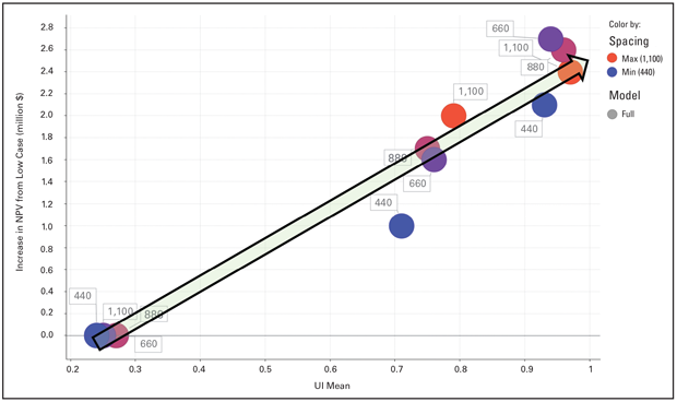
Going from the low-case UI to the high-case UI that represents a near-perfect frac stage generally increases NPV by about $2.5 million. Even starting at the base case UI and moving to the high case adds $1 million for each well. While the exact numbers for each UI group vary with well spacing, the trends are consistent. Every 0.1 improvement in UI is likely to increase first-year production about 2.5% and add about $300,000 in NPV.

Practical Implications

The detailed hydraulic fracture and reservoir simulations show that improving UI results in material increases in production and NPV. These simulations do not capture all the benefits of real-time optimization, but they offer a basis for evaluating the potential value of AIF and other ongoing efforts to improve completion effectiveness. Although the modeling is specific to the Bakken, the learnings likely apply to other unconventional reservoirs.

Given recent advances in limited entry perforating designs, we must ask how much better the industry can get at improving proppant distribution’s uniformity. Based on Hess’ DAS data, which puts the average UI around 0.75, it would be easy to assume the maximum opportunity for improvement is 0.25.

In truth, the industry likely has a much larger opportunity to unlock additional value by improving proppant distribution. One study comparing DAS measurements to perforation erosion estimates based on images from ultrasonic downhole cameras found DAS readings to be optimistic, overpredicting UI by 0.1-0.2. If that observation generalizes, Hess’ UIs could be as low as 0.55, meaning the company may improve UIs as much as 0.45 by achieving a perfect UI.

True perfection will likely remain out of reach given the complexities of stress shadowing, proppant erosion, etc. However, even if UI caps at 0.90, we still have an opportunity to increase UI by 0.15-0.35.

If the DAS measurements hold and UI only can be improved from 0.75 to 0.90, the potential value is about $450,000 for each well. But if today’s UI is still at 0.55, the value of reaching 0.90 exceeds $1 million per well.

That incremental revenue adds up. For Hess, which plans to drill more than 100 wells a year in the near term, it translates to at least $45 million a year if the company succeeds at realizing its vision for AIF and optimizing proppant distribution. Doing so will mean overcoming numerous complexities and hurdles, which will take time. Fortunately, the modeling studies also show that even modest gains in uniformity, such as the ones from ongoing improvements to limited entry designs, can create significant value.

Editor’s Note: The preceding article is the second in a two-part series that began in AOGR’s August issue. Both articles are adapted from URTeC 4044071, a technical paper presented at the 2024 Unconventional Resources Technology Conference, held June 17-19 in Houston. The full paper includes appendices that provide more details on the fully coupled model and its calibration process, as well as an in-depth comparison of the fully coupled and simple models. The authors acknowledge the contributions of the paper’s co-authors: Hess Corp.’s Michael McKimmy and John Lassek, and ResFrac Corp.’s Ankush Singh.